Background:
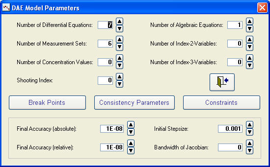
Six reactions of a batch reactor are modeled together with one algebraic
balance equation of index 1.
The Mathematical Model:
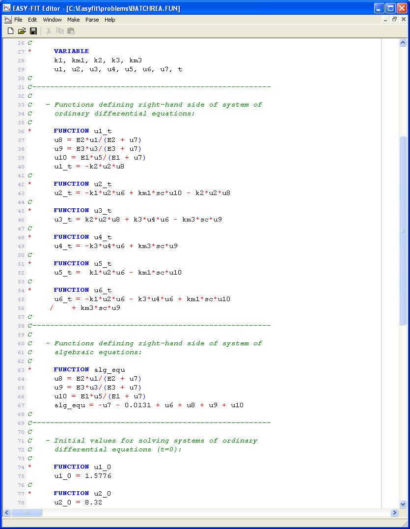
The differential state variables are denoted by u1(t) , ..., u6(t),
and the algebraic variable by u7(t) . Parameters to be
estimated, are k1, km1, k2, k3,
and km3. We define
u8(t) =
E2 u1(t) /(E2 + u7(t)
)
u9(t) = E3 u3(t)
/(E3 + u7(t) )
u10(t) = E1 u5(t) /(E1
+ u7(t) )
The six differential equations and the algebraic equation are
u1(t)t
= -k2 u2(t) u8(t)
u2(t)t
= -k1 u2(t) u6(t)
+ km1 u10(t)
- k2 u2(t)
u8(t)
u3(t)t
= k2 u2(t)
u8(t)
+ k3 u4(t)
u6(t) -
km3 u9(t)
u4(t)t
= -k3 u4(t)
u6(t) +
km3 u2(t)
u5(t)t
= k1 u2(t)
u6(t)
- km1 u10(t)
u6(t)t
= -k1 u2(t)
u6(t) -
k3 u4(t)
u6(t) +
km1 u10(t)
+ km3 u9(t)
-u7(t)
+ u6(t)
+ u8(t)
+ u9(t)
+ u10(t) = 0.0131
with initial values
u1(0) = 1.5776, u2(0) = 8.32 u3(0) =
0, u4(0) = 0, u5(0) = 0, and u6(0) =
0.0131. For
u7(0), a consistent initial value can be found. The lower index t
denotes the time derivative of the state variables.
Literature:
1. Schittkowski (2002):
Numerical Data Fitting in Dynamical Systems - A Practical Introduction with
Applications and Software,
Kluwer
Academic Publishers
2. Caracotsios M., Stewart W.E. (1985): Sensitivity analysis of Initial
values: Problems with mixed ODEs and algebraic equations, Computers and
Chemical Engineering, Vol. 9, No. 4, 359-365
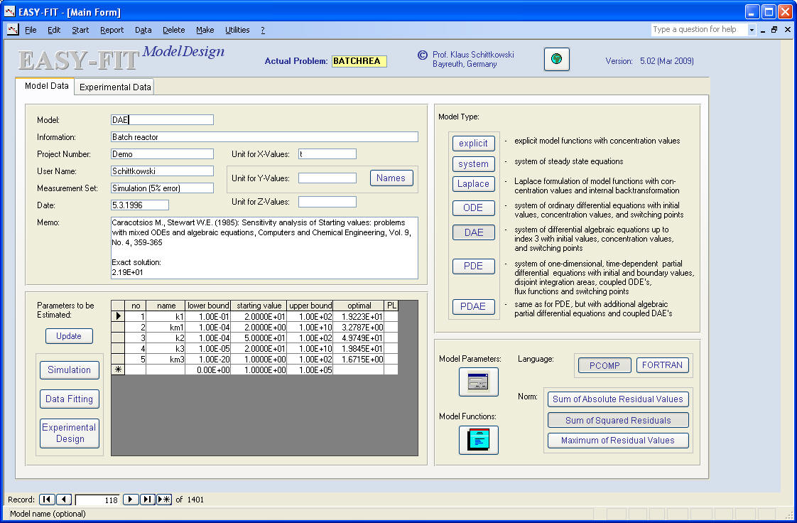
Implementation:
The complete solution of a data fitting problem is described
in six
steps:
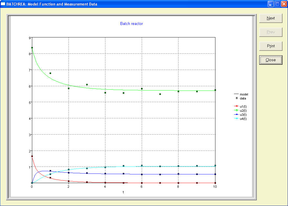
Results:
Then you would like to take a look at reports and graphs:
- parameter values
- experimental data versus fitting criterion
Model equations (or use your own favorite editor):
Measurement data (or use import function for text files or Excel):
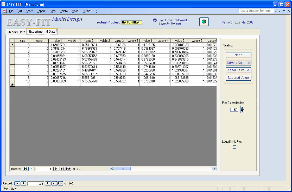
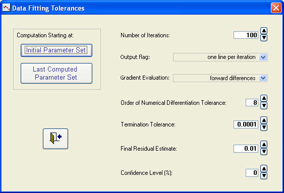
Parameters, tolerances, and start of a data fitting run:
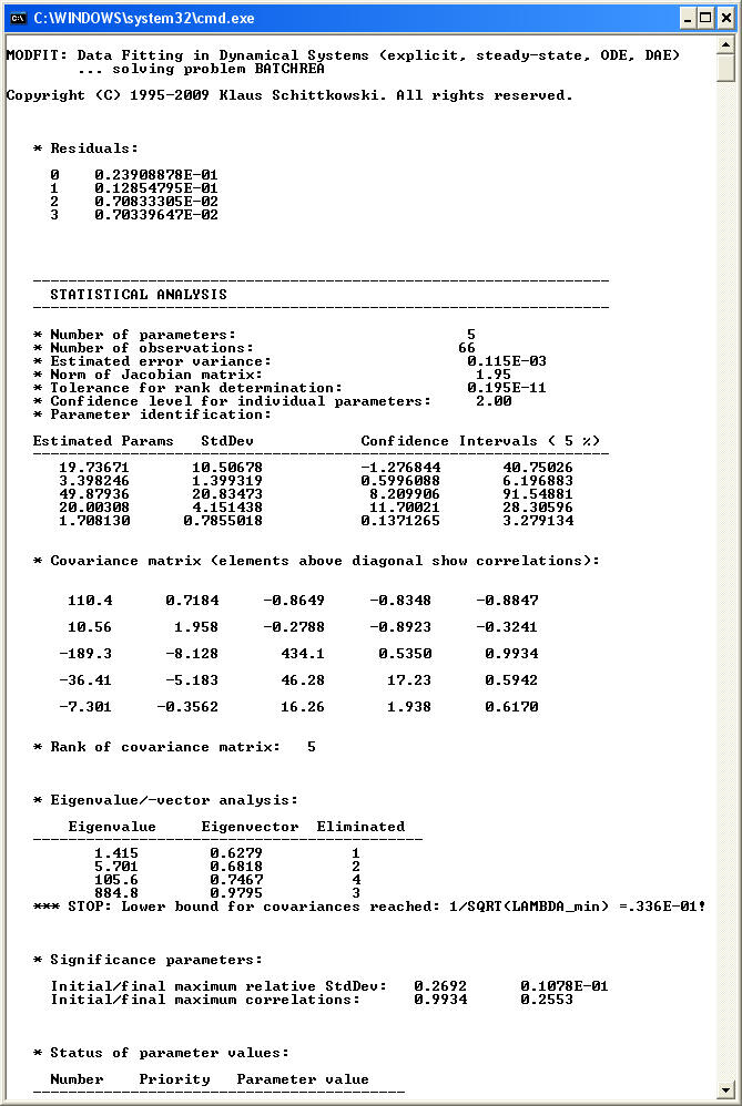
Numerical results (computed by the least squares code DFNLP):
Report on parameter values, residuals, performance, etc. (or export to Word):
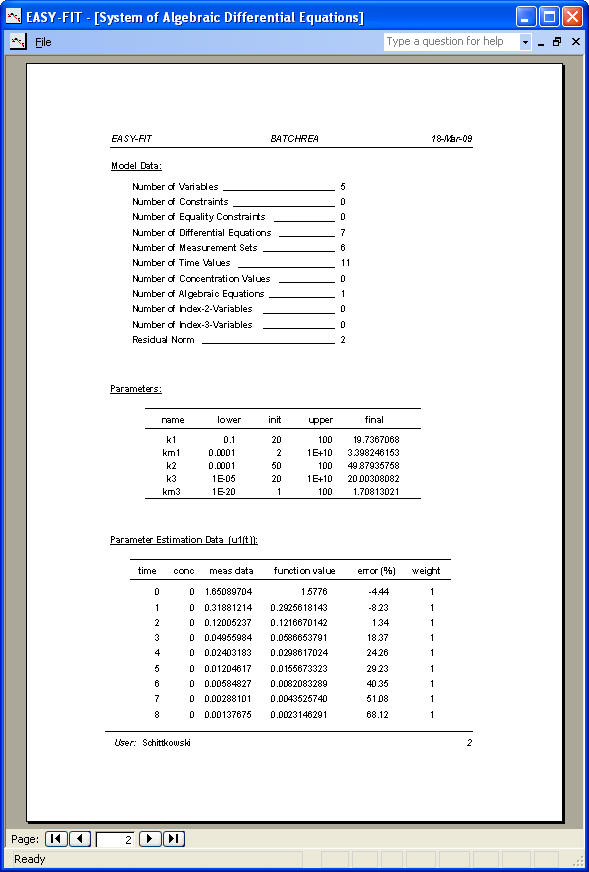
Experimental data versus fitting criterion (also available for Gnuplot):