Example: Heat equation (HEAT_A)

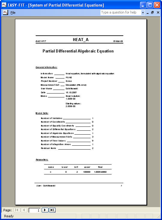
Background:
We consider a very simple partial differential equation, the heat equation describing the heat transfer in a solid rod.  In this case, the structure of a system of partial differential algebraic equations is to be outlined.

The Mathematical Model:
The one-dimensional diffusion equation is given in the form

 u(x,t)_t  =  u(x,t)_xx

The subindices 't' and 'xx', respectively, denote the partial differentiation with respect to time variable t and spatial variable x varying between 0 and 1. We suppose inhomogeneous initial value  u(x,0) = sin(p x)  and homogeneous Dirichlet boundary conditions x(0,t) = x(1,t) = 0. c is the unknown parameter to be estimated. Fitting criteria for which measurements are generated, are  u(0.25,t) , u(0.5,t) , and  u(0.75,t). In this simple situation, the explicit solution is known,

u(x,t)  = exp(-t p²) sin(x p )  

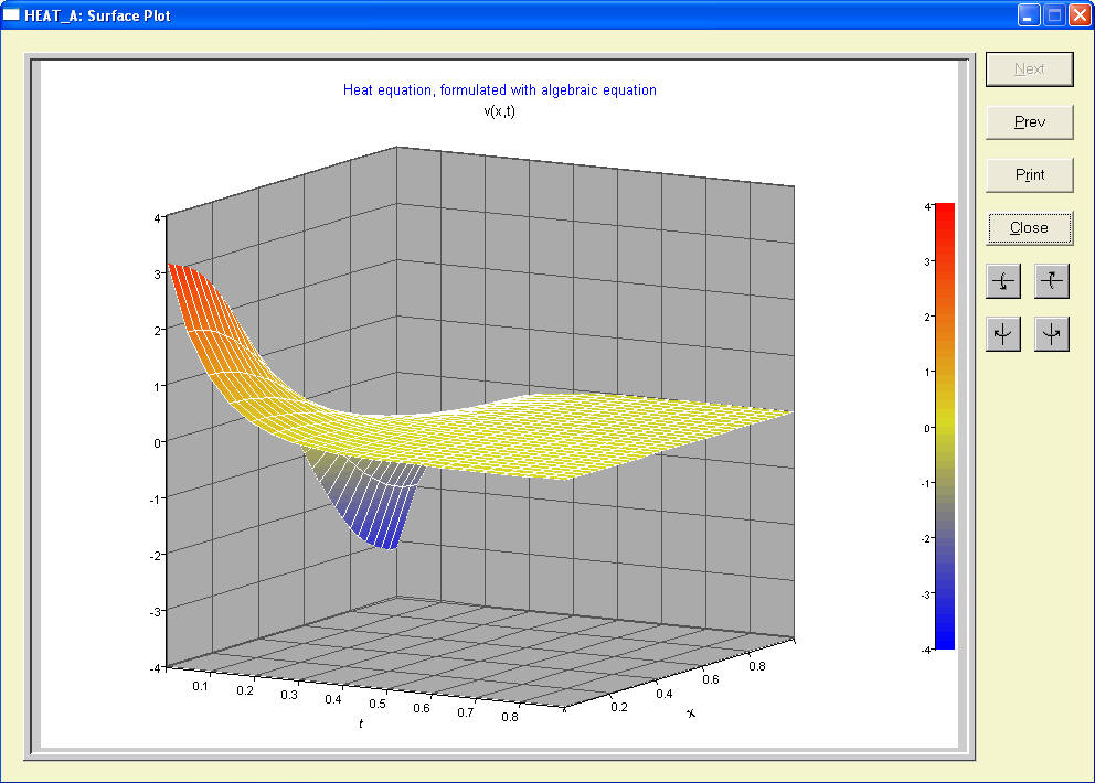
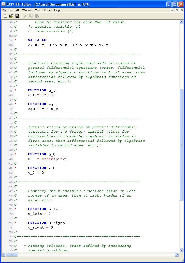
Now we introduce another, so-called algebraic state variable v(x,t), and replace above equation by

 u(x,t)_t  =  v(x,t)_x

v(x,t)  =  u(x,t)_x

An additional homogeneous initial value  v(x,0) = 0  is defined, but only for formal reasons. Consistent initial values are computed internally by PDEFIT at the grid points. Now we introduce a heat transfer coefficient c and consider the equation u(x,t)_t  =  c v(x,t)_x with initial value u(x,0) = c sin(p x). c is the unknown parameter to be estimated with true value c=1. Fitting criterion for which measurements are generated, is u(0.5,t).

Literature:
Schittkowski (2002): Numerical Data Fitting in Dynamical Systems - A Practical Introduction with Applications and Software, Kluwer Academic Publishers  

Implementation:
The complete solution of a data fitting problem is described in six steps:

1. Define model type and document the experiment
   ... set some informative strings, define the mathematical structure and the variables
2. Specify details of the model structure
   ... set number of equations, boundary values, integration tolerances, ...
3. Use editor for declaring variables and for defining functions
   ... the essential part, you have to know the mathematical equations and how to relate them to the format required by EASY-FIT^ModelDesign
4. Insert measurement data
   ... the dirty job, can become boring (but you may import data from text files and EXCEL spreadsheets!) 
5. Select termination tolerances and start a data fitting run
   ... only a few mouse clicks
6. A separate process is started and all computed data are displayed
   ... PDEFIT estimates parameters and performs a statistical analysis

Results:
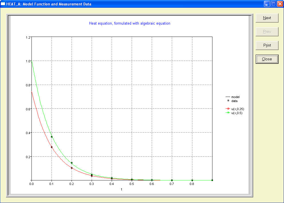
Then you would like to take a look at reports and graphs:
    - parameter values
   - experimental data versus fitting criterion
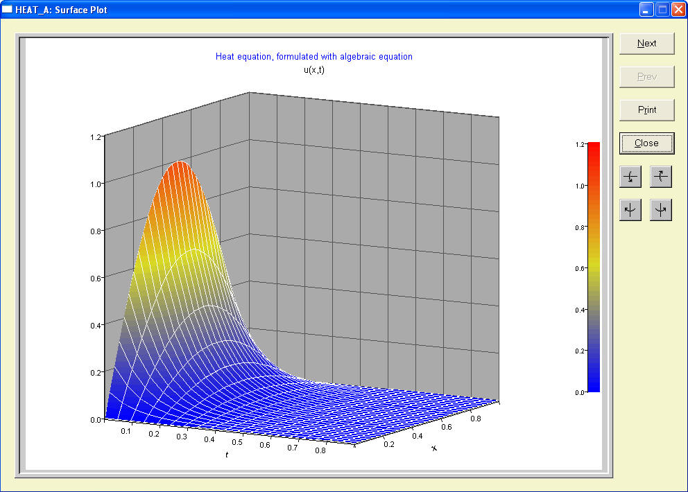
   - surface plot of state variable

Documentation and parameters:

Model structure:

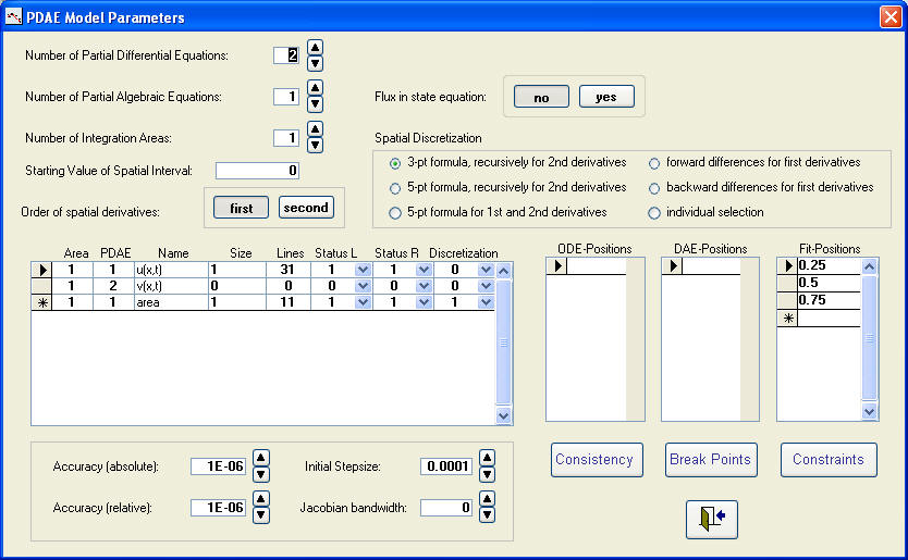
Model equations (or use your own favorite editor):

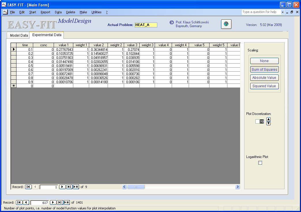
Measurement data (or use import function for text file or Excel):

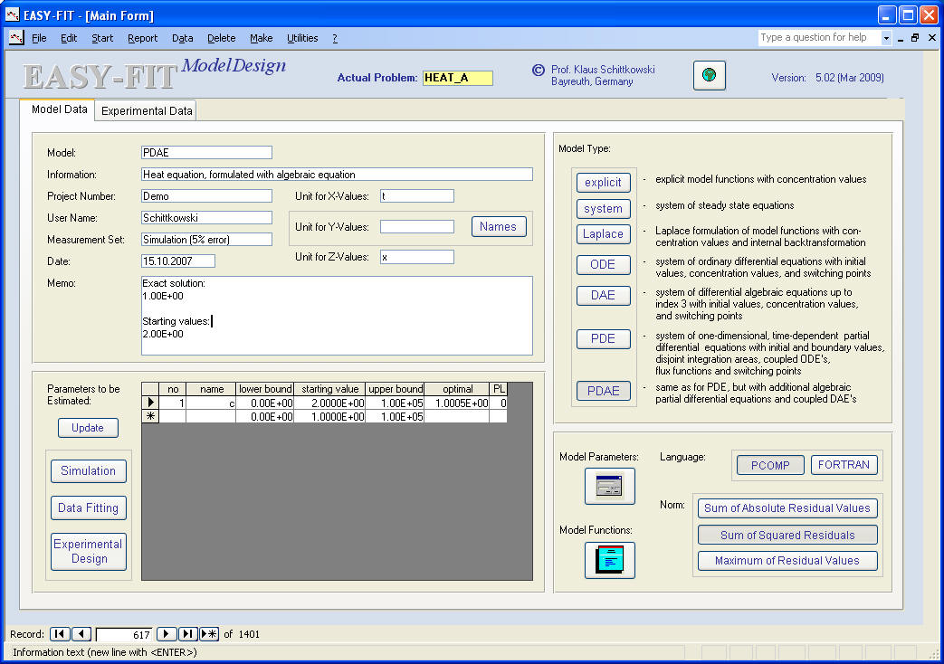
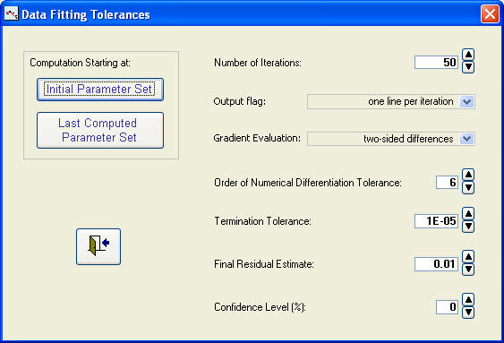
Parameters, tolerances, and start of a data fitting run:

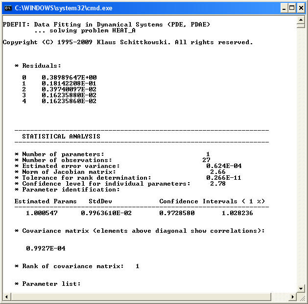
Numerical results (computed by the least squares code DFNLP):

Report about parameter values, residuals, performance, etc. (or export to Word):

Experimental data versus fitting criterion (also available for Gnuplot):

Surface plot of state variable (also available for Gnuplot):

Back to home page	Back to EASY-FIT	klaus@schittkowski.de