Example: Linear compartment model with bolus application (LKIN_L) 

Background:
The simple linear pharmakokinetic model could describe for example the time-dependent concentrations of plasma and urine based on a simple bolus application.

The Mathematical Model:
The underlying ordinary differential equation is

y₁(t)_t  =  -k_iy₁(t) 

y₂(t)_t  =  k_iy₁(t) -  k₂y₂(t)

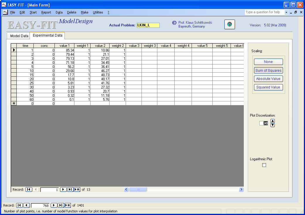
with initial values  y₁(0)=D, the initial dose, and  y₂(0)=0. Parameters to be estimated, are the rate constants  k_i and  k₂, and the dose D. Experimental data are available for  y₁(t) and y₂(t) for 13 time values between 1 min and 60 min. The lower index t denotes the time derivative of the concentrations  y₁(t) and y₂(t).

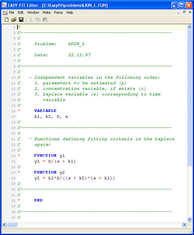
The equations can be transformed into the Laplace space, and back-transformation is done internally,

 y₁(t)  =  D/(s + k₁)

y₂(t) = k₁ D/((s+ k₁) (s+k₂))
 

Literature:
1. Heinzel G., Woloszczak R., Thomann P. (1993): TOPFIT 2.0: Pharmacokinetic and Pharmacodynamic Data Analysis System, G. Fischer, Stuttgart, Jena, New York
2. Schittkowski (2002): Numerical Data Fitting in Dynamical Systems - A Practical Introduction with Applications and Software, Kluwer Academic Publishers  

Implementation:
The complete solution of a data fitting problem is described in six steps:

1. Define model type and documentation
   ... .. set some informative strings, define the mathematical structure and the variables
2. Specify details of the model structure
   ... set number of measurement sets and concentration values in the Laplace space
3. Use editor for declaring variables and for defining functions
   ... the essential part, you have to know the mathematical equations and how to relate them to the format required by EASY-FIT^ModelDesign
4. Insert measurement data
   ... the dirty job, can become boring (but you may import data from text files and EXCEL spreadsheets!) 
5. Select termination tolerances and start a data fitting run
   ... only a few mouse clicks
6. A separate process is started and all computed data are displayed
   ... MODFIT estimates parameters and performs a statistical analysis

Results:
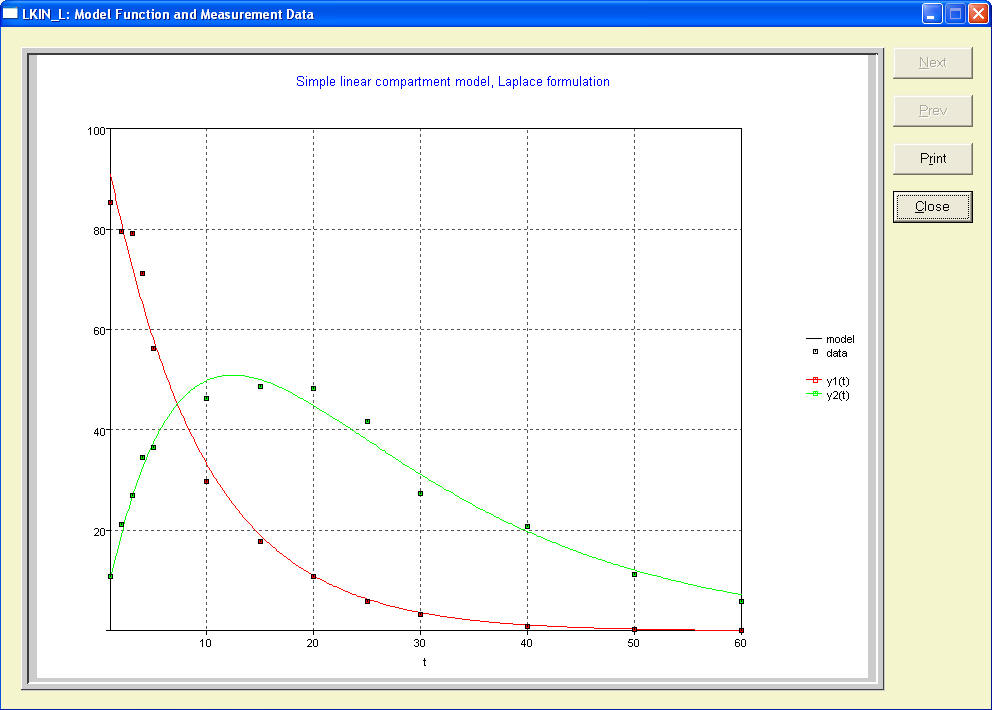
Then you would like to take a look at reports and graphs:
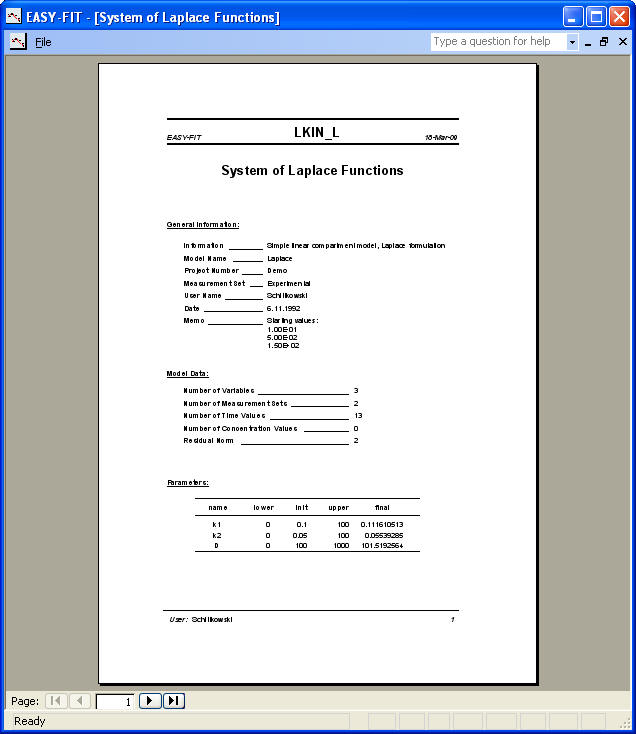
    - parameter values
   - experimental data versus fitting criterion
 

Documentation and parameters:

Model structure:

Model equations (or use your own favorite editor):

Measurement data (or use import function for text file or Excel):

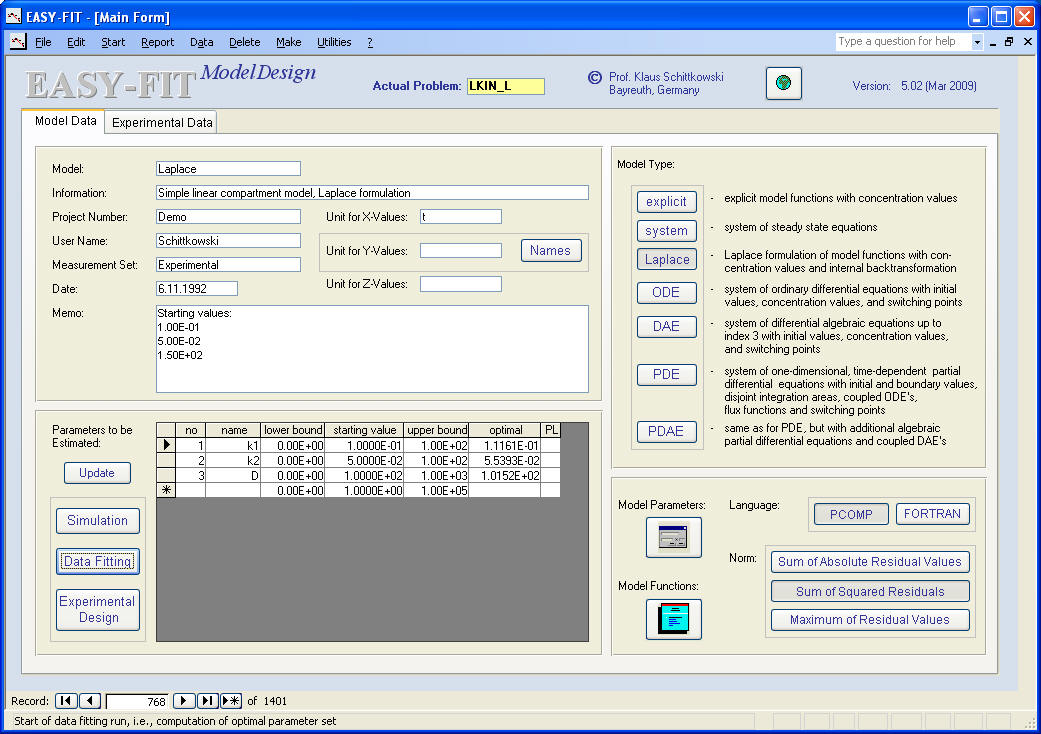
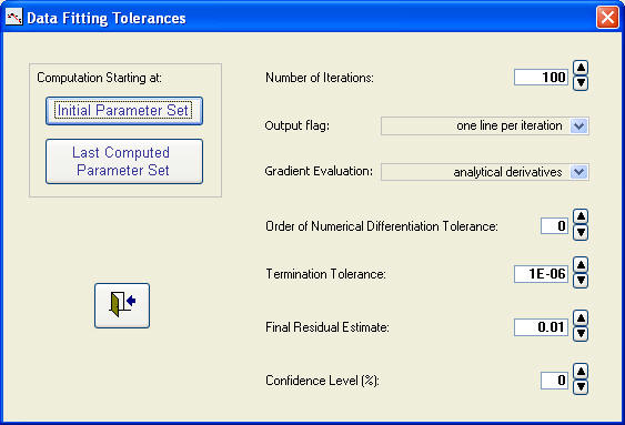
Parameters, tolerances and start of a data fitting run:

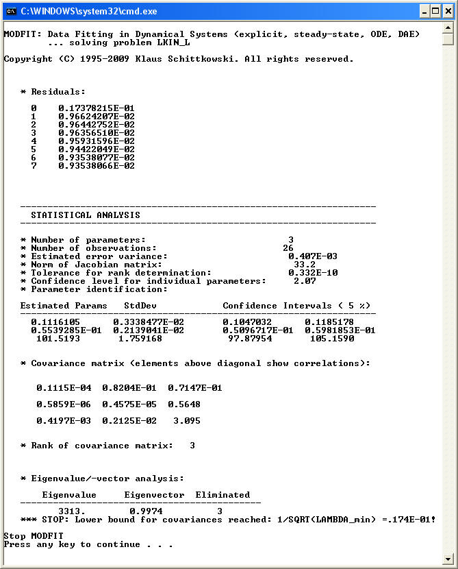
Numerical results (computed by the least squares code DFNLP):

Report on parameter values, residuals, performance, etc. (or export to Word):

Experimental data versus fitting criterion (also available for Gnuplot):

Back to home page	Back to EASY-FIT	klaus@schittkowski.de