Background:
The plain pendulum is the classical example to illustrate higher-order
differential algebraic equations. Especially, the model is able to generate
the drift effect, if modeled as a lower index system.
The Mathematical Model:
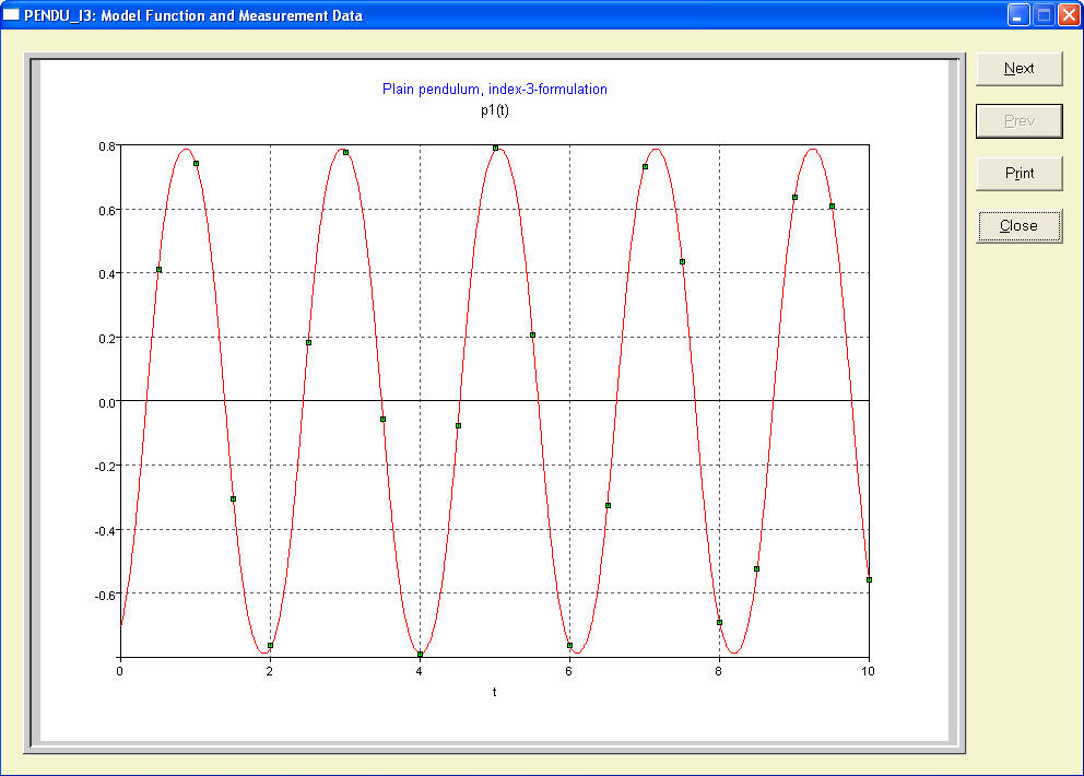
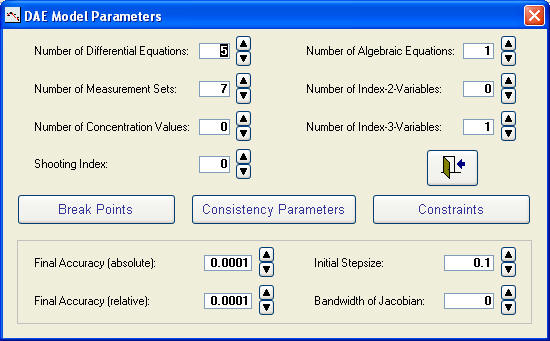
The differential state variables are denoted by p1(t) and
p2(t) for the coordinates and v1(t)
and v2(t) for the velocities. There is one algebraic variable
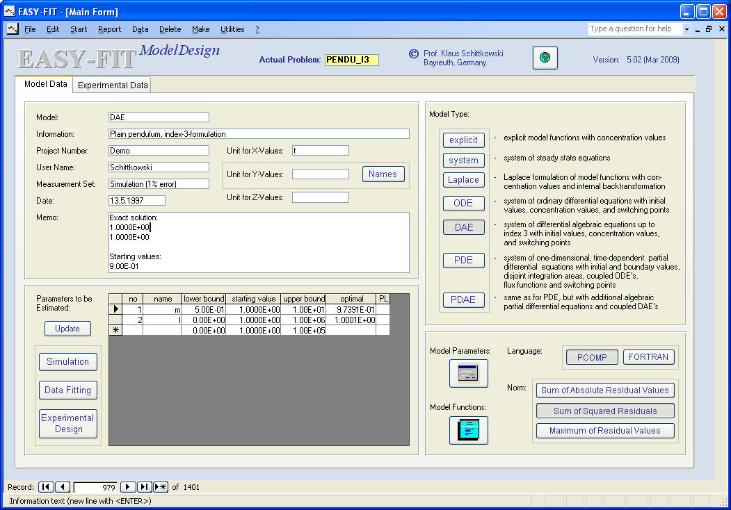
l(t). Parameters to be
estimated, are the mass m and the length l. The differential
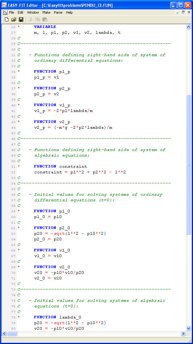
equations are
p1(t)t
= v1(t)
p2(t)t
= v2(t)
v1(t)t
= -2 p1(t) l(t) /m
v2(t)t
= (-m g -2 p2(t)
l(t))/m
One algebraic equation is needed to enforce that the mass point of the pendulum remains on a cycle,
p1(t)2 + p2(t)2 - l2 = 0
Initial positions and velocities are given, and a consistent initial value can be derived for the algebraic variable. g denotes the gravitational constant. Measurements are generated subject to an error of 1 % between 0 and 10.
Literature:
Schittkowski (2002):
Numerical Data Fitting in Dynamical Systems - A Practical Introduction with
Applications and Software,
Kluwer
Academic Publishers
Implementation:
The complete solution of a data fitting problem is described
in six
steps:
Results:
Then you would like to take a look at reports and graphs:
- parameter values
- experimental data versus fitting criterion
Model equations (or use your own favorite editor):
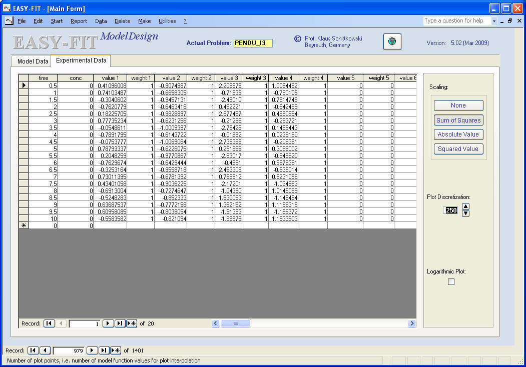
Measurement data (or use import function for text files or Excel):
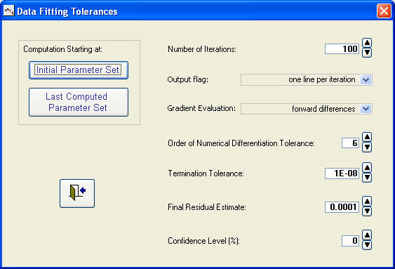
Parameters, tolerances, and start of a data fitting run:
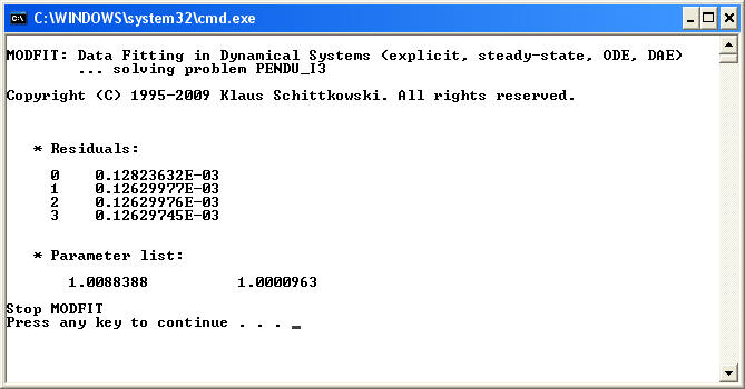
Numerical results (computed by the least squares code DFNLP):
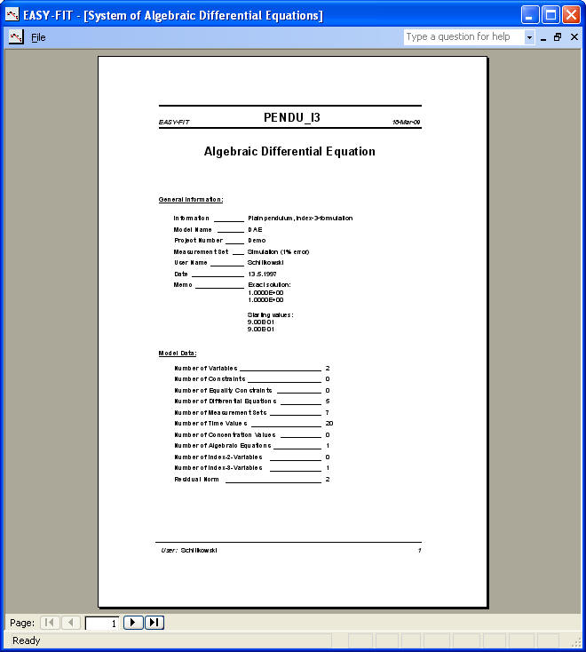
Report on parameter values, residuals, performance, etc. (or export to Word):
Experimental data versus fitting criterion (also available for Gnuplot):