Example: Diffusion of tracer through soil (SOIL)

Background:
The mathematical model describes a tracer experiment that was conducted at the lake Gaardsjon in Sweden, to investigate acidification of groundwater pollution. To conduct the experiment, a catchment of 1.000 m² was covered by a roof. A tracer impulse consisting of Lithium-Bromide was applied with steady state flow conditions. Tensiometer measurements of the tracer concentration were documented in a distance of 40 m from the center of the covered area.
 

The Mathematical Model:
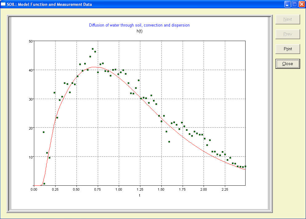
The diffusion equations proposed by Van Genuchten and Wierenga are chosen to analyze the diffusion process and to get a simulation model. A two-domain approach was selected in form of two equations, to model the mobile and the immobile part of the system. The first one is needed for the so-called immobile part, that is the mass transfer orthogonal to the flow direction, and the second one describes the diffusion of the flow through the soil by convection and dispersion:

C_im(x,t)_t  =  p_im(C_m(x,t)  -  C_im(x,t))  

C_m(x,t)_t  =  D_m C_m(x,t)_xx  -  V_m C_m(x,t)_x  -  p_m(C_m(x,t) - C_im(x,t))

The subindices 't' and 'x' or 'xx', respectively, denote the partial differentiation with respect to time variable t and space variable x. We suppose homogeneous initial values  C^im(x,0) = C_m(x,t) = 0  and boundary conditions of the form 

V_m (C_m(0,t)  -  C₀)  -  D_m C_m(0,t)_x  =  0    ,   if   t < t₀ ,

 

V_m C_m(0,t)  -  D_m C_m(0,t)_x  =  0       ,   otherwise ,

V_m C_m(L,t)  +  D_m C_m(L,t)_x  =  0       

at the right boundary x=L . C_m(x,t) and C_im(x,t) are the tracer concentrations, D_m is the dispersion coefficient, and V_m the volume. D_m, p_m, and p_im are the unknown parameters to be estimated. Fitting criterion for which measurements are available, is

V_m C_m(L/2,t)  -  D_m C_m(L/2,t)

Literature:
1. Andersson F., Olsson B. eds. (1985): Lake Gadsjon. An Acid Forest Lake and its Catchment, Ecological Bulletins, Vol. 37, Stockholm
2. Schittkowski (2002): Numerical Data Fitting in Dynamical Systems - A Practical Introduction with Applications and Software, Kluwer Academic Publishers  

Implementation:
The complete solution of a data fitting problem is described in six steps:

1. Define model type and document the experiment
   ... set some informative strings, define the mathematical structure and the variables
2. Specify details of the model structure
   ... set number of equations, boundary values, integration tolerances, ...
3. Use editor for declaring variables and for defining functions
   ... the essential part, you have to know the mathematical equations and how to relate them to the format required by EASY-FIT^ModelDesign
4. Insert measurement data
   ... the dirty job, can become boring (but you may import data from text files and EXCEL spreadsheets!) 
5. Select termination tolerances and start a data fitting run
   ... only a few mouse clicks
6. A separate process is started and all computed data are displayed
   ... PDEFIT estimates parameters and performs a statistical analysis

Results:
Then you would like to take a look at reports and graphs:
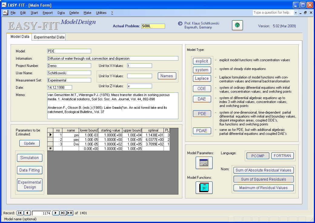
    - parameter values
   - experimental data versus fitting criterion
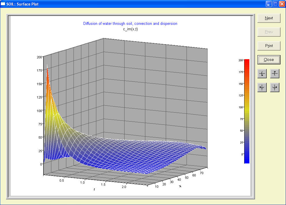
   - surface plot of state variable

Documentation and parameters:

Model structure:

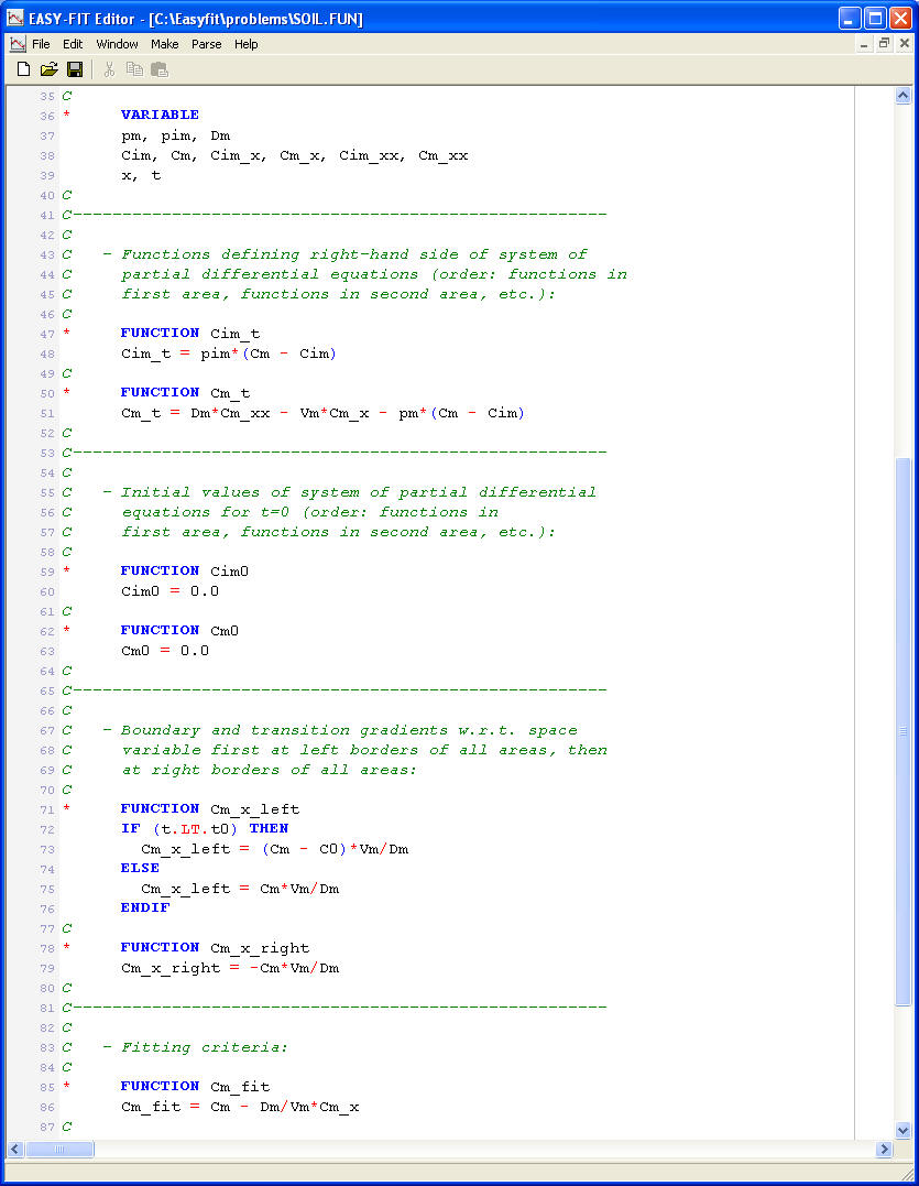
Model equations (or use your own favorite editor):

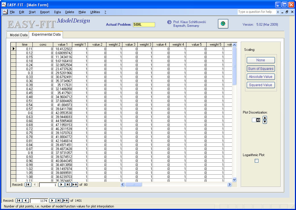
Measurement data (or use import function for text file or Excel):

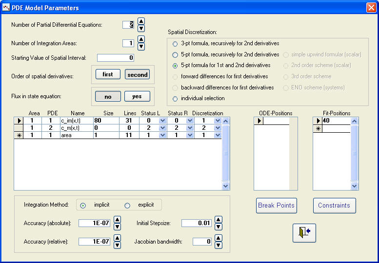
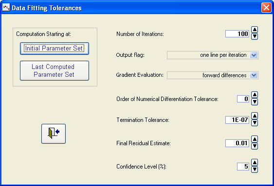
Parameters, tolerances, and start of a data fitting run:

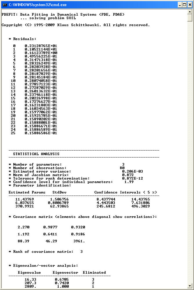
Numerical results (computed by the least squares code DFNLP):

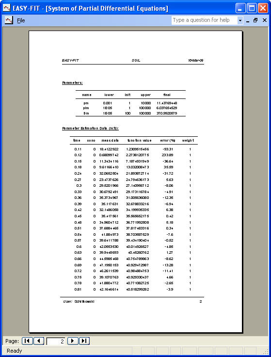
Report about parameter values, residuals, performance, etc. (or export to Word):

Experimental data versus fitting criterion (also available for Gnuplot):

Surface plot of state variable (also available for Gnuplot):

Back to home page	Back to EASY-FIT	klaus@schittkowski.de